Guideline: Decision Points

INTRODUCTION - BASIC PRINCIPLES OF BOOLEAN ALGEBRA

With almost every system, there are decision points, where the system behaviour can go in different directions, depending on the outcome of such a decision point.

The various conditions collectively determine the outcome of the decision point. The way in which a condition contributes to the outcome is reflected in terms such as “AND” or “OR”. There is a special kind of mathematics – Boolean algebra, or proposition logic – for the manipulation of these types of constructions. This chapter employs the theory of Boolean algebra, but the intention is not to instruct on this, and the interested reader is referred to the countless books on this subject. Below are the most important basic principles of Boolean algebra that are necessary for the techniques for covering decision points.

Take, for example, the following decision point that consists of only one condition: IF (number of books > 8) THEN extra discount

Decision points that consist of such singular conditions lead to two test situations, namely the situation in which the condition is true and the situation in which the condition is false. In Boolean algebra, 0 is used to indicate that something is false; 1 is used if something is true. In our example, this refers to the following test situations:

Test situation	1	2
Number of books	> 8	≤ 8
Result	True (1)	False (0)

Decision points can also consist of combinations of conditions, the so-called compound condition. Compare the following compound conditions:

IF ( Number of books > 8 OR sum ≥ €250 ) THEN extra discount
and
IF ( Number of books > 8 AND sum ≥ €250 ) THEN extra discount

Often an abbreviation is used by replacing the conditions by a capital letter (A, B, etc.) The two decision points mentioned above are thus abbreviated to:

A OR B and
A AND B

A compound condition is also either true or false, depending on the truth values of the individual conditions and the way in which the conditions are connected (the so-called operators): by an AND or an OR. With two conditions, the following combinations are possible:

A	B
1	1
1	0
0	1
0	0

This is called the complete decision table.

In the 0-0 situation, both statements are false. In the 0-1 situation and the 1-0 situation, only one of the two statements is true and in the 1-1 situation, both are true. The end result in each of the 4 situations depends on the operator “AND” or “OR”: with an “AND” the end result of two conditions is only true if both individual conditions are true; in all the other cases, the end result is false. With an “OR” the reverse is the case: the end result is only false if both individual conditions are false; in all the other cases the end result is true.

A common way of demonstrating the outcomes of all the situations of a complete decision table is the truth table. Below shows the truth tables for the compound conditions “A OR B” and “A AND B”.

A	B	A OR B
1	1	1
1	0	1
0	1	1
0	0	0

A	B	A AND B
1	1	1
1	0	0
0	1	0
0	0	0

For a decision point that consists of, not two, but three conditions, the complete decision table is as follows:

A	B	C
1	1	1
1	1	0
0	1	1
0	1	0
1	0	1
1	0	0
0	0	1
0	0	0

Clearly, the number of situations increases exponentially with the number of conditions. With 6 conditions, there are already 64 situations. Where there is a mixture of operators (AND and OR) in a compound condition, the outcome depends on which operator is executed first. To avoid confusion, it is best to indicate this by using brackets. In the absence of brackets, the rule is that the AND goes before the OR. As an example, the truth table is shown below for the compound condition “(A OR B) AND C”.

A	B	C	(A OR B) AND C
1	1	1	1
1	1	0	0
0	1	1	1
0	1	0	0
1	0	1	1
1	0	0	0
0	0	1	0
0	0	0	0

Although many different Boolean operators exist, it appears that every operator can be brought back to a combination of 3 elementary operators: AND, OR and NOT. That means that if the tester knows how to deal with these 3 operators, he can tackle every decision point. (The operator “NOT” is not dealt with here; the effect of this operator is insignificant: the outcome “1” is converted to “0” and vice versa.)

THE COMMONEST COVERAGE TYPES IN RELATION TO DECISION POINTS

The complete decision table defines all possible combinations of the individual conditions. Therefore, the testing of all these possibilities is the most thorough coverage type in respect of a decision point, and is known as “multiple condition coverage”. In addition, there are various coverage types with which a subset of the complete decision table is tested. This does not refer to a random subset, but to a subset with a specific goal. Table 1 describes in brief the commonest coverage types and their comparative degree of thoroughness. A more thorough coverage type ‘implies’ a less thorough coverage type, i.e.: one that covers minimally all the test situations of the elementary coverage type.

Condition coverage	The possible outcomes of (“true” or “false”) for each condition are tested at least once.
Decision coverage	The possible outcomes of the decision are tested at least once.
Condition/decision coverage	The possible outcomes of each condition and of the decision are tested at least once. This implies both “condition coverage” and “decision coverage”.
Modified condition/ decision coverage	Every possible outcome of a condition determines at least once the outcome of the decision. This implies “condition/decision coverage”.
Multiple condition coverage	All the possible combinations of outcomes of conditions in a decision (therefore the complete decision table) are tested at least once. This implies “modified condition/decision coverage”.

Table 1: Overview of the commonest coverage types in relation to decision points.

Take the following decision point as an example: IF (number of books > 8 OR sum ≥ €250) THEN extra discount. The tables below show with which situations the relevant coverage type is obtained.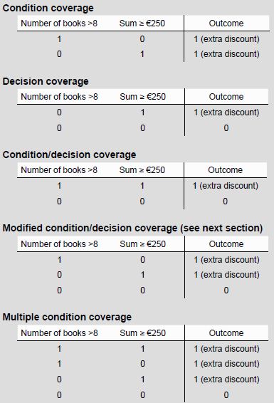

With some coverage types, other choices of situations are possible that lead to the same goal. For example, condition coverage is also achieved with the 2 situations “1 1” and “0 0”. And decision coverage is also achieved with “1 0” and “0 0” (and also with “1 1” and “0 0”).

For the most elementary coverage type, the best choice is “condition/decision coverage”, which fulfils both “condition coverage” and “decision coverage”, and requires the same number of test situations.

The coverage type “modified condition/decision coverage” is a very powerful means of obtaining thorough coverage with a small number of test situations. This coverage type is not readily mastered by everyone. For that reason, it is explained in depth in the following section.

Modified condition/decision coverage

"Modified condition/decision coverage (abbreviation: MCDC) is the coverage type that guarantees the following: Every possible outcome of a condition is the determinant of the outcome of the decision at least once."

The important concept in this definition is “determinant”. If the outcome of the condition changes (from 0 to 1 or vice versa) then the outcome of the whole decision point changes with it. The meaning of MCDC can be explained as follows:

If a decision point consists of the conditions A, B and C, then MCDC guarantees:

That there is at least 1 test situation in which the outcome is TRUE, owing to the fact that condition A is TRUE
That there is at least 1 test situation in which the outcome is FALSE, owing to the fact that condition A is FALSE
Ditto for condition B and ditto for condition C

This is a thorough level of coverage, with which the following faults, for example, would be detected in the system under test:

There is a condition missing that should be present
The “AND” was wrongly implemented as an “OR”, and vice versa
A condition has been inverted, such as “<” instead of “>” or “≠” instead of “=”.

The big advantage of this coverage type is its efficiency: with a decision point that consists of N conditions, usually only N+1 test situations are required for MCDC. Compared with the maximum number of test situations (the complete decision table) of 2N , that is a considerable reduction, particularly if N is large (complex decision points). This combination of “thorough coverage” with “relatively few test situations” makes this coverage type a powerful weapon in the tester’s arsenal.

According to the definition of MCDC, every condition should determine the outcome of the decision once. Then all the other conditions in that situation should be given a value that has no influence on the outcome of the decision. This value is called the “neutral value” and is further explained below.

Take, for example, the complex decision (R), which consists of a combination of two conditions (A, B). The outcome of the decision is only true if both conditions are true. In other words: R = A AND B

Now suppose that condition B is FALSE (or value 0). Then it no longer matters what A is; the outcome of R is always FALSE. In other words: A AND 0 = 0

However, if condition B is TRUE (or value 1), the R outcome of the decision depends entirely on the outcome of A. In other words: A AND 1 = A

This last is exactly what should be achieved with MCDC: If condition A should determine the outcome of the decision (in this ‘AND combination’), then the other condition should be set at value 1. We are talking here about the neutral value, since value 1 has no influence on the final outcome.

Similarly, we can talk of the neutral value for the ‘OR combination’, which is 0 in this
case, since: A OR 0 = A

In summary: The neutral value with AND = 1. The neutral value with OR = 0.

6-step plan for deriving test situations for MCDC

Employing the concept of “neutral value”, achieving MCDC can be translated in concrete terms into the requirements:

Let every condition within the decision be TRUE once and FALSE once,
With all the other conditions in that test situation being given a neutral value.

There are various ways of deriving the necessary test situations. The 6-step plan is a technique that very directly follows on the definition of MCDC and with which a table is simply created with all the necessary test situations. The 6-step plan is explained below with a relatively simple example. Subsequently, it is explained how this technique works for more complex combinations of conditions.

Take as an example the following decision point, which describes how good customers receive an extra discount: IF (Number of books > 8 OR Sum ≥ €250) THEN extra discount

The decision point here is made up of 2 conditions with the structure: R = A OR B.

The 6-step plan is set out below, giving the test situations with which this decision point is covered by MCDC.

1. Create a table with 3 columns.

Fill in the first row as follows:

R = A OR B

2. Add 1 row for every condition in the decision.

This row will contain the 2 test situations in which the relevant condition determines the outcome of the decision point. The condition will decide the outcome “1” once and the outcome “0” once. In the first column, enter the description of every condition.

R = A OR B	1	0
A: Number of books > 8
B: Sum ≥ €250

3. Fill in the rest of the cells in the table with a number of dots equal to the number of conditions in the decision. Each cell is a test situation, which should indicate which combination of TRUE/FALSE applies to the conditions.

R = A OR B	1	0
A: Number of books > 8	..	..
B: Sum ≥ €250	..	..

4. Enter “1” diagonally in the second column and “0” in the third column. This is actually entering the determining values for every condition. The meaning of e.g. the cell that belongs to row “A” and column “1” is: “This is the test situation in which condition A determines an outcome of 1.”

R = A OR B	1	0
A: Number of books > 8	1 .	0 .
B: Sum ≥ €250	. 1	. 0

5. Over the remaining dots, enter a neutral value. In this case, both A and B will contribute to the outcome via an OR combination. So for both, the neutral value is 0.

R = A OR B	1	0
A: Number of books > 8	1 0	0 0
B: Sum ≥ €250	0 1	0 0

6. Score out duplicates of test situations.

R = A OR B	1	0
A: Number of books > 8	1 0	0 0
B: Sum ≥ €250	0 1	~~0 0~~

The 6-step plan described above works for every compound condition, however complex. With compound conditions in which both “AND” and “OR” occur, care should be taken at step 5 (entering the neutral values). The example below will explain this.

Take as an example the decision point R = (A OR B) AND C. After the first 4 steps, the table of test situations looks as follows:

R = (A OR B) AND C	1	0
A	1 . .	0 . .
B	. 1 .	. 0 .
C	. . 1	. . 0

Now the neutral values should be entered for each of the 6 situations. With the top 2 situations (A is the determining value), the neutral values can immediately be determined: B is connected to A via the operator “OR” and should therefore be given the neutral value “0”. C is connected with A via the operator “AND” and should therefore be given the neutral value “1”.

The same applies to the middle 2 situations (B is the determining value). However, for the bottom situation (C is the determining value) an interim step is necessary: it is not A that is directly connected with C, nor is it B. It is the combination “(A OR B)” that is connected with C, via the operator “AND”. Thus “(A OR B)” should assume the neutral value of “AND”, and that is “1”. In other words: (A OR B) = 1. For the values for A and B there are 3 possibilities of achieving this, i.e. “1 1”, “1 0” or “0 1”. Only 1 of the 3 need to be selected to reach the goal of MCDC. In principle, it does not matter which. The only difference in the 3 possibilities is that in selecting “1 0” or “0 1” a test situation can be scored off, while that is not possible with the choice of “1 1”.

If the neutral value of “1 0” is selected for (A OR B), then after the 6 steps, the table looks as follows:

R = (A OR B) AND C	1	0
A	1 0 1	0 0 1
B	0 1 1	~~0 0 1~~
C	~~1 0 1~~	1 0 0

This phenomenon, that several possibilities exist for neutral values, always occurs in cases of an operator between brackets.